dodgr isochrones, isodists, and isoverts

Mark Padgham

2025-10-13

The dodgrpackage includes three functions for calculating iso-contours from one or more points of origin:

• dodgr_isodists() for contours of equal distance;
• dodgr_isochrones() for contours of equal time; and
• dodgr_isoverts() to return full set of vertices within defined isodistance or isochrone contours.

Each of these functions is fully vectorised to accept both multiple origin points and multiple contours. Each returns a single data.frame object, with a column specifying either the distance or time limit (as dlim for dodgr_isodists(), or tlim for dodgr_isochrones()). The functions are also internally parallelised for efficient calculation.

Input formats

The dodgr_isodists() function accepts arbitrary input, either as a generic dodgr data.frame (with a “distance” column), or as street networks derived from applying the weight_streetnet() function to either sf or st objects. Time-based calculations in dodgr are only possible when applied to street networks dervied from st objects, because equivalent sf-based objects can only provide crude estimates of journey times. The time-specific functions dodgr_isochrones() and dodgr_isoverts() thus only accept dodgr street networks derived from sc data. The following table summarises the requirements of these functions:

Function	Input type
dodgr_isodists	Either sf or sc format data
dodgr_ isochrones	Only sc format data
dodgr_isoverts	Only sc format data

dodgr_isodists

The dodgr_isodists() function calculates contours of equal distance from one or more points of origin.

graph <- weight_streetnet (hampi)
from <- sample (graph$from_id, size = 100)
dlim <- c (2, 5, 10, 20) * 100
d <- dodgr_isodists (graph, from = from, dlim)
dim (d)

## [1] 2573    5

knitr::kable (head (d))

from	dlim	id	x	y
4506481411	200	4506481406	76.46174	15.31509
4506481411	200	4506481416	76.45951	15.31643
4506481411	200	4506481411	76.46081	15.31590
4506481411	200	4506481406	76.46174	15.31509
4506481411	500	4506481406	76.46174	15.31509
4506481411	500	4506481416	76.45951	15.31643

This function returns in this case a data.frame with the columns shown above and 2,573 points defining the isodistance contours from each origin (from) point, at the specified distances of 200, 500, 1000, 2000 metres. There are naturally more points defining the contours at longer distances:

table (d$dlim)

## 
##  200  500 1000 2000 
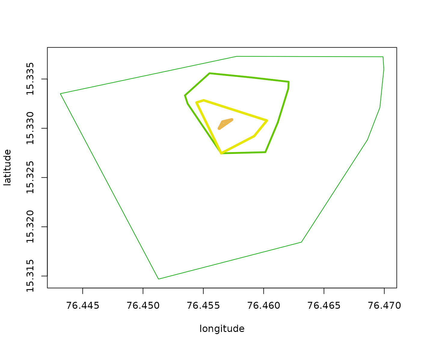
##  406  578  716  873

The points defining the contours are arranged in an anticlockwise order around each point of origin, and so can be directly visualised using base graphics functions. This is easier to see by using just a single point of origin:

set.seed (1)
from <- sample (graph$from_id, size = 1)
dlim <- c (2, 5, 10, 20) * 100
d <- dodgr_isodists (graph, from = from, dlim)
cols <- terrain.colors (length (dlim) + 2) # + 2 to avoid light colours at end of scale.
index <- which (d$dlim == max (d$dlim)) # plot max contour first
plot (
    d$x [index], d$y [index], "l",
    col = cols [1],
    xlab = "longitude", ylab = "latitude"
)
for (i in seq (dlim) [-1]) {
    index <- which (d$dlim == rev (dlim) [i])
    lines (d$x [index], d$y [index], col = cols [i], lwd = i + 1)
}

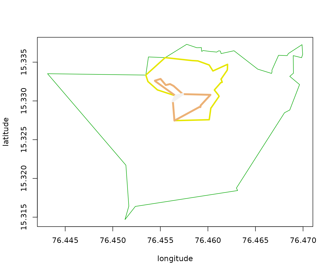
The concavity parameter

The default contours are convex hulls. The dodgr_isodists() and dodgr_isochrones() functions include an additional concavity parameter to return generate concave isodistance or isochrone polygons, defaulting to a value of 0 for no concavity. Changing this value can generate concave contours like in the following results:

set.seed (1)
from <- sample (graph$from_id, size = 1)
dlim <- c (2, 5, 10, 20) * 100
d <- dodgr_isodists (graph, from = from, dlim, concavity = 0.5)
cols <- terrain.colors (length (dlim))
index <- which (d$dlim == max (d$dlim))
plot (
    d$x [index], d$y [index], "l",
    col = cols [1],
    xlab = "longitude", ylab = "latitude"
)
for (i in seq (dlim) [-1]) {
    index <- which (d$dlim == rev (dlim) [i])
    lines (d$x [index], d$y [index], col = cols [i], lwd = i + 1)
}

The calculation of isodists or isochrone values is cached, so different values of the concavity parameter can be trialled without needing to re-calculate the underlying values:

set.seed (2)
from <- sample (graph$from_id, size = 1)
dlim <- c (2, 5, 10, 20) * 100
system.time ( # Initial call calculates distances to all points:
    d <- dodgr_isodists (graph, from = from, dlim, concavity = 0.5)
)

##    user  system elapsed 
##   0.160   0.001   0.161

system.time ( # Subsequent call uses cached values:
    d <- dodgr_isodists (graph, from = from, dlim, concavity = 0.75)
)

##    user  system elapsed 
##   0.022   0.000   0.022

The concavity parameter has a default value of 0 for strictly convex polygons. Values closer to 1 generate more concave polygons. The following code demonstrates the effect of increasing values of this parameter.

set.seed (5)
from <- sample (graph$from_id, size = 1)
dlim <- 2000
concavity <- 0:4 / 4
d <- lapply (concavity, function (i) dodgr_isodists (graph, from = from, dlim, concavity = i))
cols <- terrain.colors (length (d) + 2)
plot (
    d [[1]]$x, d [[1]]$y,
    type = "l",
    col = cols [1], lwd = 5,
    xlab = "longitude", ylab = "latitude"
)
for (i in seq_along (d) [-1]) {
    lines (
        d [[i]]$x, d [[i]]$y,
        col = cols [i], lwd = 6 - i, lty = i
    )
}
v <- dodgr_vertices (graph)
v_from <- v [match (from, v$id), ]
points (v_from [, c ("x", "y")], pch = 19, col = "red", cex = 2)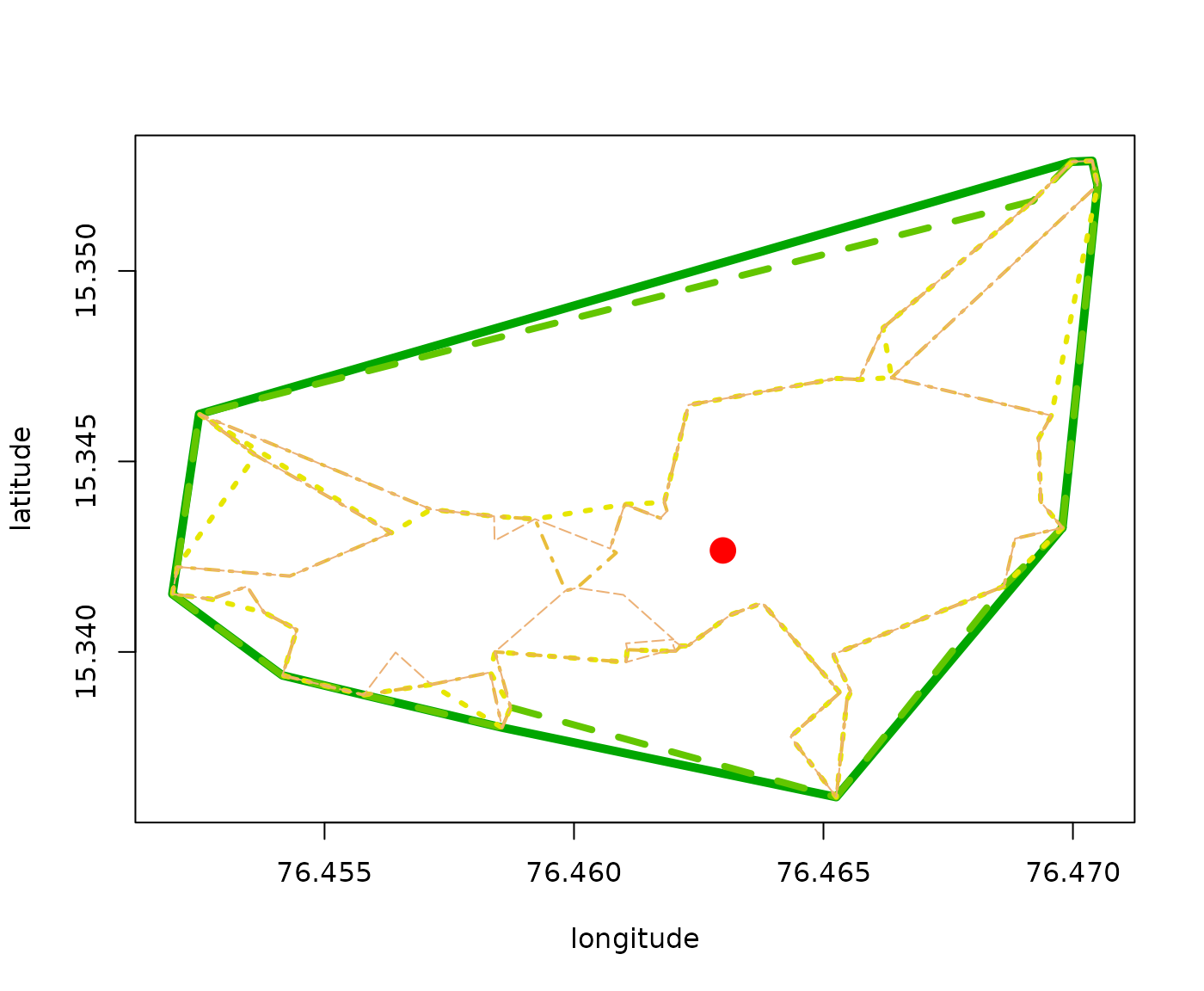

dodgr_isochrones

The dodgr_isochrones() works just like dodgr_isodists() except that it can only be applied to street networks generated from silicate (SC) format data. The results differ only from equivalent distance results in having a column named “tlim” (for “time”) instead of “dlim” (for “distance”). The concavity parameter functions in exactly the same way as described above.

dodgr_isoverts

Both the dodgr_isodists() and dodgr_isochrones() functions work by estimating distances or times from specified origin points to all points out to the maximum specified values of dlim or tlim. A second stage then generates convex or concave hulls around these points, with the result containing an ordered sequence of points tracing the contours around these hulls.

The dodgr_isoverts() function generates the full underlying set of points without applying any hull-tracing routines. This resultant points may be used, for example, to apply some custom hull-tracing routine, or to perform statistical analyses on the full points enclosed within specified values of dlim or tlim. The object returned from this function is identical to those demonstrated above, with a column named “dlim” if the dlim parameter is specified, or “tlim” if the tlim parameter is specified. The data.frame returned from dodgr_isoverts() will always contain more data, and have more rows, than equivalent results from dodgr_isodists() or dodgr_isochrones(). The rows of the data.frame returned from dodgr_isoverts() are ordered by increasing dlim or tlim values, but rows for any given value of those parameters are in arbitrary order. Each successively higher value of either dlim or tlim includes all points denoted by all lower values. For example, all values contained within dlim = 200 are all those with that specified value of dlim plus all rows with any values of dlim < 200.

The following code demonstrates typical sizes of results from the dodgr_isodists() and dodgr_isoverts() functions:

dat <- dodgr_streetnet_sc ("hampi india")
graph <- weight_streetnet (dat, wt_profile = "foot")
set.seed (1)
from <- sample (graph$.vx0, size = 1)
dlim <- c (2, 5, 10, 20) * 100
nrow (dodgr_isodists (graph, from = from, dlim))

## [1] 34

nrow (dodgr_isoverts (graph, from = from, dlim))

## [1] 145